Introduction¶

The dl_esm_inf (for Daresbury Laboratory Earth-System Modelling Infrastructure) library provides basic support for finite-difference earth-system-type models written in Fortran. It currently supports two-dimensional, finite-difference models.

The first version of this library was developed to support 2D finite- difference shallow-water models in the GOcean Project.

Grid¶

The dl_esm_inf library contains a grid_mod module which defines a grid_type and associated constructor:

use grid_mod
...
!> The grid on which our fields are defined
type(grid_type), target :: model_grid
...
! Create the model grid
model_grid = grid_type(GO_ARAKAWA_C,                                 &
                       (/GO_BC_EXTERNAL,GO_BC_EXTERNAL,GO_BC_NONE/), &
                       GO_OFFSET_NE)

Note

The grid object itself must be declared with the target attribute. This is because each field object will contain a pointer to it.

The grid_type constructor takes three arguments:

The type of grid (only GO_ARAKAWA_C is currently supported)

The boundary conditions on the domain for the x, y and z dimensions (see below). The value for the z dimension is currently ignored.

The ‘index offset’ - the convention used for indexing into offset fields.

Three types of boundary condition are currently supported:

Name	Description
GO_BC_NONE	No boundary conditions are applied.
GO_BC_EXTERNAL	Some external forcing is applied. This must be implemented by a kernel. The domain must be defined with a T-point mask (see The grid_init Routine).
GO_BC_PERIODIC	Periodic boundary conditions are applied.

The infrastructure requires this information in order to determine the extent of the model grid.

The index offset is required because a model (kernel) developer has choice in how they actually implement the staggering of variables on a grid. This comes down to a choice of which grid points in the vicinity of a given T point have the same array (i, j) indices. In the diagram below, the image on the left corresponds to choosing those points to the South and West of a T point to have the same (i, j) index. That on the right corresponds to choosing those points to the North and East of the T point (this is the offset scheme used in the NEMO ocean model):

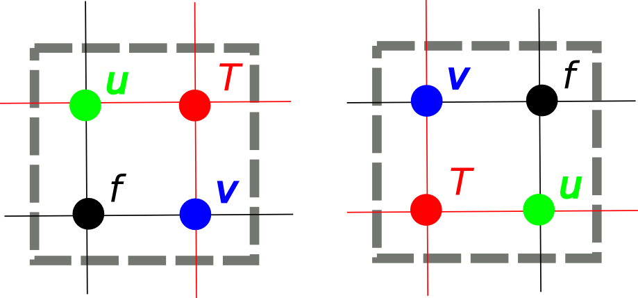
The GOcean 1.0 API supports these two different offset schemes, which we term GO_OFFSET_SW and GO_OFFSET_NE.

Note that the constructor does not specify the extent of the model grid. This is because this information is normally obtained by reading a file (a namelist file, a netcdf file etc.) which is specific to an application. Once this information has been obtained, a second routine, grid_init, is provided with which to ‘load’ a grid object with state. This is discussed below.

The `grid_init` Routine¶

Once an application has determined the details of the model configuration, it must use this information to populate the grid object. This is done via a call to the grid_init subroutine:

subroutine grid_init(grid, m, n, dxarg, dyarg, tmask)
  !> The grid object to configure
  type(grid_type), intent(inout) :: grid
  !> Dimensions of the model grid
  integer,         intent(in)    :: m, n
  !> The (constant) grid spacing in x and y (m)
  real(wp),        intent(in)    :: dxarg, dyarg
  !> Optional T-point mask specifying whether each grid point is
  !! wet (1), dry (0) or external (-1).
  integer, dimension(m,n), intent(in), optional :: tmask

If no T-mask is supplied then this routine configures the grid appropriately for an all-wet domain with periodic boundary conditions in both the x- and y-dimensions. It should also be noted that currently only grids with constant resolution in x and y are supported by this routine.

Fields¶

The field constructor method¶

Once a model has a grid defined it will require one or more fields. dl_esm_inf contains a field_mod module which defines an r2d_field type (real, 2-dimensional field) and associated constructor:

use field_mod
...
!> Current ('now') sea-surface height at different grid points
type(r2d_field) :: sshn_u_fld, sshn_v_fld, sshn_t_fld
...

! Sea-surface height now (current time step)
sshn_u = r2d_field(model_grid, GO_U_POINTS)
sshn_v = r2d_field(model_grid, GO_V_POINTS)
sshn_t = r2d_field(model_grid, GO_T_POINTS)

The constructor takes two arguments:

The grid on which the field exists

The type of grid point at which the field is defined (GO_U_POINTS, GO_V_POINTS, GO_T_POINTS or GO_F_POINTS)

Note that the grid object must have been fully configured (by a call to grid_init for instance) before it is passed into this constructor.

Device infrastructure attributes¶

The fields have some infrastructure capabilities to allow the allocation of the data in different memory regions (usually acceleration devices but it can also be a user provided data layout on the same host) and manage the synchronization between the original data and the device data.

These capabilities are provided by the following field attributes:

field_type%data_on_device: A boolean to indicate if the data has already been allocated and copied in the device.
field_type%read_from_device_f or field_type%read_from_device_c: Function pointers that provide the synchronization method to copy the data back from the device into the host. The user needs to provide one of these function pointers implemented in the programming model of choice. The Fortran and C function pointers need to have the following interfaces, respectively:
Fortran:
abstract interface
  subroutine read_from_device_f_interface(from, to, nx, ny, width)
    use iso_c_binding, only: c_intptr_t, c_int
    use kind_params_mod, only: go_wp
    integer(c_intptr_t), intent(in) :: from
    real(go_wp), dimension(:,:), intent(inout) :: to
    integer, intent(in) :: nx, ny, width
  end subroutine read_from_device_f_interface
end interface
C:
abstract interface
  subroutine read_from_device_c_interface(from, to, nx, ny, width)
      use iso_c_binding, only: c_intptr_t, c_int
      integer(c_intptr_t), intent(in), value :: from
      integer(c_intptr_t), intent(in), value :: to
      integer(c_int), intent(in), value :: nx, ny, width
  end subroutine read_from_device_c_interface
end interface
r2d_field%device_ptr: A pointer to the device memory location where the copy of the field’s data is located.

These attributes do not conform to any specific device programming model with the idea that the specific model details are provided by the infrastructure user. See below an example using the FortCL library:

use field_mod
use FortCL, only: create_rw_buffer
...
!> Declare and initialize the field
type(r2d_field) :: sshn_t
sshn_t = r2d_field(model_grid, GO_T_POINTS)
...

sshn_t%device_ptr = create_rw_buffer(size_in_bytes)
sshn_t%data_on_device = .true.
sshn_t%read_from_device_f = read_function

...

! Code using sshn_t%device_ptr
...

! The data will be copied back from the device to the host at this point
write(*,*) sshn_t%get_data(10,10)

contains

subroutine read_function(from, to, nx, ny, width)
  use FortCL, only: read_buffer
  use iso_c_binding, only: c_intptr_t, c_int
  integer(c_intptr_t), intent(in) :: from
  real(go_wp), dimension(:,:), intent(inout) :: to
  integer, intent(in) :: nx, ny, width
  ! Use width instead of nx in case there is padding elements
  call read_buffer(from, to, int(width*ny, kind=8))
end subroutine read_fortcl

Example¶

In what follows we walk through a slightly cut-down example of the use of the dl_esm_inf library.

The following code illustrates the use of the library in constructing an application:

program gocean2d
  use grid_mod  ! From dl_esm_inf
  use field_mod ! From dl_esm_inf
  use model_mod
  use boundary_conditions_mod

  !> The grid on which our fields are defined. Must have the 'target'
  !! attribute because each field object contains a pointer to it.
  type(grid_type), target :: model_grid

  !> Current ('now') velocity component fields
  type(r2d_field) :: un_fld, vn_fld
  !> 'After' velocity component fields
  type(r2d_field) :: ua_fld, va_fld
  ...

  ! time stepping index
  integer :: istp

  ! Create the model grid. We use a NE offset (i.e. the U, V and F
  ! points immediately to the North and East of a T point all have the
  ! same i,j index).  This is the same offset scheme as used by NEMO.
  model_grid = grid_type(GO_ARAKAWA_C,                                &
                        (/GO_BC_EXTERNAL,GO_BC_EXTERNAL,GO_BC_NONE/), &
                         GO_OFFSET_NE)

  !! read in model parameters and configure the model grid
  CALL model_init(model_grid)

  ! Create fields on this grid

  ! Velocity components now (current time step)
  un_fld = r2d_field(model_grid, GO_U_POINTS)
  vn_fld = r2d_field(model_grid, GO_V_POINTS)

  ! Velocity components 'after' (next time step)
  ua_fld = r2d_field(model_grid, GO_U_POINTS)
  va_fld = r2d_field(model_grid, GO_V_POINTS)

  ...

  !! time stepping
  do istp = nit000, nitend, 1

    call step(istp,                               &
              ua_fld, va_fld, un_fld, vn_fld,     &
              ...)
  end do
  ...
end program gocean2d

The model_init routine is application specific since it must determine details of the model configuration being run, e.g. by reading a namelist file. An example might look something like:

subroutine model_init(grid)
  type(grid_type), intent(inout) :: grid

  !> Problem size, read from namelist
  integer :: jpiglo, jpjglo
  real(wp) :: dx, dy
  integer, dimension(:,:), allocatable :: tmask

  ! Read model configuration from namelist
  call read_namelist(jpiglo, jpjglo, dx, dy, &
                     nit000, nitend, irecord, &
                     jphgr_msh, dep_const, rdt, cbfr, visc)

  ! Set-up the T mask. This defines the model domain.
  allocate(tmask(jpiglo,jpjglo))

  call setup_tpoints_mask(jpiglo, jpjglo, tmask)

  ! Having specified the T points mask, we can set up mesh parameters
  call grid_init(grid, jpiglo, jpjglo, dx, dy, tmask)

  ! Clean-up. T-mask has been copied into the grid object.
  deallocate(tmask)

end subroutine model_init

Here, only grid_type and the grid_init routine come from the dl_esm_inf library. The remaining code is all application specific.

Once the grid object is fully configured and all fields have been constructed, a simulation will proceed by performing calculations with those fields. In the example program given above, this calculation is performed in the time-stepping loop within the step subroutine.

Introduction¶

Grid¶

The `grid_init` Routine¶

Fields¶

The field constructor method¶

Device infrastructure attributes¶

Example¶

dl_esm_inf

Navigation

Related Topics

Introduction¶

Grid¶

The grid_init Routine¶

Fields¶

The field constructor method¶

Device infrastructure attributes¶

Example¶

The `grid_init` Routine¶